- Calc III Review
- Dipoles
- Current and Conductivity
- Capacitance
- Ampere's Force Law
- Force between straight wires
- Ampere's Circuital Law
- Point form of Ampere's circuital law
- Mass spectrometer
- Magnetic field through a boundary
- Faraday's law (change in magnetic flux)
- Lenz's Law
- Power and Energy in an inductor
- Transformers
- Solenoid
- Young's Experiment
- Electromagnetic Waves
- Reflection
Calc III Review
History of Vectors
More than 10 vector systems developed between 1790 and 1850
quaternions - scalar + vector - William Hamilton
modern vectors - direction + magnitude - Gibbs and Heaviside
field - function which assigns quantity to points in space
scalar - ex. temperature in space vector - ex. electromagnetic field
spherical coordinates 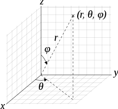
cylindrical coordinates 
Gradient
The change in each direction of a field
cartesian coordinates
\[\overrightarrow{\nabla} F = \frac{d}{dx} F_x \hat{a_x} + \frac{d}{dy} F_y \hat{a_y} + \frac{d}{dz} F_z \hat{a_z}\]
Divergence
The measure of outflow of a field in an infinitesimal volume around some point
\[ \nabla F = \lim_{V \to 0} \iint_S \frac{F \times n}{V} dS \]
Laplacian
\[\nabla \cdot \overrightarrow{\nabla} F \]
Dipoles
Bound charges
\(\overrightarrow{E_D} = \frac{\overrightarrow{D} - \overrightarrow{P}}{\varepsilon_0}\)
\[ \begin{aligned} \overrightarrow{P} &= \varepsilon_0 x_e \overrightarrow{E} \\ &= \varepsilon_0(1 + x_e)\overrightarrow{E} \end{aligned} \]
\[ \begin{aligned} \overrightarrow{D} & = \varepsilon_0 \overrightarrow{E} + \varepsilon_0 x_e \overrightarrow{E} \\ & = \varepsilon_0 (1 + x_e) \overrightarrow{E} \\ & = \varepsilon_0 \varepsilon_r \overrightarrow{E} \end{aligned} \]
Coulomb's Law in Dielectric
\[ \begin{aligned} \overrightarrow{D} &= \frac{q_2}{4\pi r^2} \hat{a_r}^2 \\ \overrightarrow{E} &= \frac{q_2}{4\pi \varepsilon_0 \varepsilon_r r^2} \hat{a_r}^2 \\ \overrightarrow{F_{1,2}} &= \frac{q_2 q_1}{4\pi \varepsilon_0 \varepsilon_r r^2} \hat{a_r}^2 \end{aligned} \]
Current and Conductivity
The current density \(J\) in a conductive material is the amount of current flowing perdendicular through a unit area
\(J = u \rho_c q\)
where \(u\) is the velocity of the particles, \(\rho_c\) is the density of the particles, and \(q\) is the charge per particle
The conductivity \(\sigma\) of a material relates the strength of the electric field to the current flowing per cross sectional area
\(\overrightarrow{J} = \sigma \overrightarrow{E}\)
Current flow from applied voltage
Let a voltage \(V\) be applied to a conductive block with cross-sectional area \(A\) and length \(d\).
Then the total current flow is \(I = \frac{\sigma V A}{d}\)
Resistances in series
Let a conductive block have cross-sectional area \(A\) and length \(2d\). There are two conductive regions in series with conductivities \(\sigma_1, \sigma_2\)
\(R_{tot} = R_1 + R_2 = \frac{d}{A \sigma_1} + \frac{d}{A \sigma_2}\)
Capacitance
For a charged body, the work required to approach the body scales with charge,
so the ratio between charge and voltage is constant, called capacitance
\(C = \frac{Q}{V}\)
Capacitance of parallel plate capacitor

\(C = \frac{Q}{V} = \frac{\varepsilon_0 \varepsilon_r A}{d}\)
Capacitances in parallel

\(C_T = C_1 + C_2\)
Energy in Capacitor
\(W = \frac{1}{2} CV^2\)
Changing capacitor shape
Assume a capacitor is charged to some voltage, and the voltage is removed. The charge on the plates will remain, regardless of how the plates are moved.
If the distance between the plates is doubled, \(\overrightarrow{E}\) remains constant, so:
\(V = - \int_0^d \overrightarrow{E} dl = dE\) -> \(V = - \int_0^{2d} \overrightarrow{E} dl = 2dE\)
and the voltage is doubled.
Examples
Solve for \(E_2\)

\(D = \frac{Q}{A} = E_1 \varepsilon_1 = E_2 \varepsilon_2\)
\(E_1 = E_2 \frac{\varepsilon_2}{\varepsilon_1}\)
\[ \begin{aligned} V & = - \int_{d_1} \overrightarrow{E_1} \overrightarrow{dl} - \int_{d_2} \overrightarrow{E_2} \overrightarrow{dl} \\ & = - \int_{d_1} \overrightarrow{E_2} \frac{\varepsilon_2}{\varepsilon_1} \overrightarrow{dl} - \int_{d_2} \overrightarrow{E_2} \overrightarrow{dl} \\ & = d_2 E_2 + d_1 E_2 \frac{\varepsilon_2}{\varepsilon_1} \end{aligned} \]
\[E_2 = \frac{V}{d_2 + d_1 \frac{\varepsilon_2}{\varepsilon_1}}\]
A metal sphere of radius 1m is surrounded everywhere by a dielectric with \(\varepsilon_r = 3\). Find the capacitance of the sphere.

Assume a charge \(Q\) on the sphere.
\(\overrightarrow{D} = \frac{Q}{4 \pi r^2} \hat{a_{\rho}}\) (from Gauss's equation)
\[\overrightarrow{E} = \frac{\overrightarrow{D}}{\varepsilon_0 \varepsilon_r} = \frac{Q}{4 \pi \varepsilon_0 \varepsilon_r r^2} \hat{a_{\rho}}\]
\[V = V(1) - V(\infty) = \frac{Q}{4 \pi \varepsilon_0 \varepsilon_r (1)^2}\]
\[C = \frac{Q}{V} = 4 \pi \varepsilon_0 \varepsilon_r = 12 \pi \varepsilon_0\]
Ampere's Force Law
Magnetic field from point current
Magnetic Field Intensity
Contribution from point current
\[\overrightarrow{dH} = \frac{I \overrightarrow{dl} \times \hat{r'}}{4 \pi R^2} \frac{A}{m}\]
where \(\hat{r'}\) is the vector pointing from the point current to \(\overrightarrow{r}\)
\[\overrightarrow{H} = \oint \overrightarrow{dH} \frac{A}{m}\]
\[dF = \mu_0 I_1 \overrightarrow{dl_1} \times \overrightarrow{dH}\]
Force between straight wires
Magnetic flux density
\[\overrightarrow{B(\rho)} = \frac{I}{2 \pi \rho} \hat{r'}\]
Units are in \(\frac{Vs}{m^2} = \frac{Wb}{m^2} = T = 10,000 G\)
Find the force between two parallel wires with opposite currents

\[\overrightarrow{dF_1} = \mu_0 -I_1 \overrightarrow{dl} \times \frac{I_2}{2 \pi R} \hat{r'}\]
\[\overrightarrow{F_1} = \int_0^L \mu_0 (-I_1 dz \hat{a_z}) \times \frac{I_2}{2 \pi R} a_{\phi} = - \frac{\mu_0 I_1 I_2 L}{4 \pi R} \hat{r'}\]
Ampere's Circuital Law
Around current

\(\oint H \cdot \overrightarrow{dl} = I\)
Outside of current

\(\oint H \cdot \overrightarrow{dl} = 0\)
Magnetic field intensity of single wire
\(H(\rho) = \frac{I}{\rho 2 \pi}\)
Magnetic field intensity of slab of current
\[\overrightarrow{H} = \frac{Z}{2}\]
Where \(K = J \Delta H\) is called the sheet charge density

Magnetic field intensity of cylinder of current
Many point currents arranged in a circle with radius \(a\) and \(I_T = K(2 \pi)(a)\)
\[ H(\rho) = \begin{cases} \frac{I}{2 \pi \rho} & \phi \geq a,\\ 0 & \phi \leq a \end{cases} \]
Point form of Ampere's circuital law
incomplete
\(\frac{dH_y}{dx} - \frac{dH_x}{dy} = J_z\) \[ \begin{aligned} \oint \overrightarrow{H} \cdot \overrightarrow{dl} & = J_Z \Delta x \Delta y \\ \int_1^4 \overrightarrow{H} \cdot \overrightarrow{dl} + \int_2^3 \overrightarrow{H} \cdot \overrightarrow{dl} + \int_3^4 \overrightarrow{H} \cdot \overrightarrow{dl} + \int_1^2 \overrightarrow{H} \cdot \overrightarrow{dl} & = J_z \Delta x \Delta y \\ H_{14} \Delta x + H_{23} \Delta y - H_{34} \Delta x - H_{12} \Delta y = J_Z \Delta x \Delta y \\ (H_{0x} - \frac{\Delta y}{2} \frac{dH_x}{dy})\Delta x \end{aligned} \]
\(\overrightarrow{F_m} = \mu_0 (I \overrightarrow{dl} \times \overrightarrow{H})\)
\(\overrightarrow{F_m} = \mu_0 (Q\mu \times \overrightarrow{H})\)
\(\overrightarrow{F_m} = Qu \times \mu_0 \overrightarrow{H}\)
\(\overrightarrow{B} = \mu_0 \overrightarrow{H}\)
\(\overrightarrow{F_m} = Qu \times \overrightarrow{B}\)
Lorentz Force Equation \(\overrightarrow{F} = Q \overrightarrow{E} + Q\mu \times \overrightarrow{B}\)
Mass spectrometer
incomplete A particle with some known charge is fired into a chamber with a known magnetic field.
Due to the forces generated from a moving charge in a magnetic field, the particle will curve as it travels through the field.
\(\overrightarrow{F_m} = Qu \times \overrightarrow{B} = QuB(-\hat{a_{\rho}}) = m \frac{u^2}{r} \hat{a_{\rho}}\)
so \(r = \frac{mu^2}{QuB}\)
assume Si+ and As+

$KE = (100 \frac{J}{C})(1.6*10^{-19} C)$

$u(Si+) = 2.62 * 10^4 \frac{m}{s}$

$u(As+) = 1.6 * 10^4 \frac{m}{s}$

$r(Si+) = $

$r(As+) = $
Magnetic field through a boundary
Since there are no magnetic monopoles, we can determine the normal component of the magnetic field through the boundary by drawing a simple body on the boundary.
\[ \begin{aligned} B_{1N} & = B_{2N} \\ \mu_1 H_{1N} & = \mu_2 H_{2N} \end{aligned} \]
We can determine the parallel component using Ampere's circuital law with the assumption that the parallel field induces a current on the boundary.
Faraday's law (change in magnetic flux)
Experimentally, we can see that
\[i = -\frac{N}{R} \frac{d\Psi}{dt}\]
\[ \begin{aligned} V_{emf} & = iR = -N\frac{d\Psi}{dt} - \frac{d\lambda}{dt}\\ \oint \overrightarrow{E} \cdot \overrightarrow{dl} & = -N \frac{d \int \overrightarrow{B} \cdot \overrightarrow{ds}}{dt} \end{aligned} \]
where \(N\) is the number of turns in the coil, \(R\) is the total resistance, and \(\Psi\)
Or since \(L = \frac{\lambda}{i}\)
\(V_{emf} = - \frac{d\lambda}{dt} = -L \frac{di}{dt}\)
Lenz's Law
The induced current will flow in a direction that opposes the magnetic flux.
Power and Energy in an inductor
\(qV\) - energy delivered to R and L by a single charge
\(n\) - number of \(q\) moving around circuit per second
\(P = nqV = IV\) - energy delivered to R and L per second by all charges
\[ \begin{aligned} \oint \overrightarrow{E} \cdot \overrightarrow{dl} & = \frac{d\lambda}{dt} \\ -V + IR + 0 & = -L \frac{di}{dt} \end{aligned} \]
\(V = IR + L \frac{di}{dt}\)
\[ \begin{aligned} W & = \int P dt = \int iV dt = \int_0^T(iR + L i\frac{di}{dt}) dt = \int_0^T i^2 R dt + \int_0^T Li di \\ & = \frac{1}{2}Li^2 \end{aligned} \]
Transformers
Primary winding \(V_1 = \oint \overrightarrow{E} \cdot \overrightarrow{dl} = -(N_1 \frac{d\Psi}{dt})\)
\(-(N_2 \frac{d\Psi}{dt}) = \oint \overrightarrow{E} \cdot \overrightarrow{dl} = V_2\)
\(V_2 = \frac{N_2}{N_1} V_1\)
Solenoid
\(\int \overrightarrow{H} dl = I_{enc} \to A\)

\(\overrightarrow{B} = \mu \overrightarrow{H}\) (Henries)
\(B * A = \Psi\) (Henry-Amps)
\(\oint \overrightarrow{E} \cdot \overrightarrow{dl} = \frac{d}{dt} \Psi\) (Henry-Amps)/sec = V
Let \(\frac{d\Psi}{dt} = 10V\)
The reading from \(VOM_1\) and \(VOM_2\) are different. \(VOM_1\) is approximately \(10V\) since the changing magnetic field flows through the surface created by its wires.
The reading from \(VOM_2\), since the surface is not pierced by the magnetic field coming from the solenoid.
Using faraday's law,
\[ \begin{aligned} \oint \overrightarrow{E} \cdot \overrightarrow{dl} & = - \frac{d\Psi}{dt} \\ IR & = - \frac{d\Psi}{dt} = \frac{d}{dt} \left[ Blx \right] = Blxv \end{aligned} \]
\(\overrightarrow{F_m} = \int I \overrightarrow{dl} \times \overrightarrow{B} dl = IB \int_0^l dy = -IBl \hat{a_x}\)
\(\oint H \cdot dl = I_{enc}\)
Move the boundary of the surface between the plates of a capacitor.
$ =
Young's Experiment
Young demonstrated the particle and wave behavior of light with his experiment.

He shone light through a pair of narrow slits, which resulted bands forming on the photosensitive plate, suggesting wave-like behavior. This is because the distance between a band and each slit results in a slight phase shift of the light wave.
If the intensity of the light is lowered and exposure of the plate is brief, the photons hitting the plate cause specs of exposure, suggesting particle-like behavior.
Electromagnetic Waves
\[u = \frac{\omega}{\beta} = \frac{2 \pi f}{\frac{2 \pi}{\lambda}} = f \lambda = \frac{1}{\sqrt{\mu \varepsilon}} \]
\(\overrightarrow{\mathbb{P}} = \overrightarrow{E} \times \overrightarrow{H}\) - energy of waves (Poynting vector)
Plane Waves in Lossless Media
incomplete
\(\overrightarrow{E}(z,t) = E_{x0} e^{-\alpha z} \cos(\omega t - \beta z) \hat{a}_x\)
\(\overrightarrow{H}(z,t) = \frac{\varepsilon}{\mu} E_{x0} e^{-\alpha z} \cos(\omega t - \beta z) \hat{a}_y\)
\(\mu = \frac{\omega}{\beta}\) - velocity \(\beta = \frac{2 \pi}{\lambda}\) - wave number
\(n = \sqrt{\frac{\mu}{\varepsilon}}\) -
Let \(\overrightarrow{H} = 25 \cos(1.33*10^{-4}z + 40,000t) \hat{a}_y \frac{A}{m}\)
Find the wavelength:
Plane Waves in Lossy Media
\(\overrightarrow{E}(z,t) = E_0 e^{-\alpha z} \cos(\omega t - \beta z) \hat{a}_x\)
\(\overrightarrow{H}(z,t) = \frac{E_0}{n} e^{-\alpha z} \cos(\omega t - \beta z) \hat{a}_y\)
\(n = \sqrt{\frac{j \omega \mu}{\sigma + j\omega \varepsilon}}\) - intrinsic impedance
\(\alpha + j \beta = \sqrt{j \omega \mu (\sigma + j \omega \varepsilon)} = \gamma\) - propogation constant
Assume \(\mu_r = 1\). \(\overrightarrow{H} = 25 \sin(2 \times 10^8 t + 6x) \hat{a}_y\)
For the wave to hold in place * as \(t\) increases, \(x\) must decrease. So the wave propogates in the \(-\hat{a}_x\) direction.
\(\omega = 2 \times 10^8 s^{-1}\), \(\beta = 6 = \frac{2 pi}{\lambda}\),
\(u = \frac{\omega}{\beta} = \frac{2 \times 10^8}{6} \frac{m}{s} = \frac{1}{\sqrt{\mu \varepsilon}}\)
Since material is lossless, \(\mu = \mu_0\)
\(\frac{1}{3} \times 10^8 = \frac{1}{\sqrt{\mu \varepsilon}} = \frac{1}{\sqrt{\mu_0 \varepsilon_0 \varepsilon_r}}\)
so \(\varepsilon_r = 81\)
Find E. \(n = \sqrt{\frac{\mu}{\varepsilon_r}} = \frac{377}{9} \Omega\)
\(E = n H = \frac{377}{9} (25 \frac{mA}{m}) = 1.05 \frac{V}{m}\)
Using the geometry of the wave \(\overrightarrow{\cal{P}} = \overrightarrow{E} \times \overrightarrow{H}\), we can find that the direction of propogation is in the \(\hat{a}_z\) direction, so
\(\overrightarrow{E} = 1.05 \sin(2 \times 10^8 t + 6X) \hat{a}_z \frac{V}{m}\)
Let E⃗ = 16e-0.05x sin (2 × 10 8 t - 2x) âz $
Find propogation constant
\(\gamma = \alpha + Jj \beta = 0.05 + j2\)
Find λ
\(\beta = \frac{2\pi}{\lambda}\)
\(\lambda = \frac{2\pi}{\beta} = \pi\)
Find the velocity \(u\)
\(u = \frac{\omega}{\beta} = \frac{2 \times 10^8 (s^{-1})}{2 (m^{-1})} = 10^8 \frac{m}{s}\)
Find the skin depth \(\delta\)
\(\delta = \frac{1}{\alpha} = 20\)
Skin depth
If the current through the wire is increasing, current loops perpendicular to the current flow to oppose the magnetic field generated. \(\delta = \frac{1}{\alpha}\) - skin depth

Reflection
Assume non-magnetic lossless
In the first medium, \(E_i = 10 \cos(3 \times 10 ^8 t - 1z) \hat{a}_x \frac{V}{m}\), \(\varepsilon_r = 1\), \(\varepsilon_{r2} = 16\)
\(\eta_0 = \sqrt{\mu_0}{\varepsilon_0}\), \(\eta_2 = \sqrt{\mu_0}{16 \varepsilon_0}\)
Find r
\(r = \eta_2 - \eta_1}{\eta_2 + \eta_1} = -3/5\)
Find \(E_r\)
\(E_{r0} = rE_{io} = -6\)
\(E_r = -6\cos(3 \times 10^8 t - 1z) \hat{a}_x\)
Find \(E_t\)
\(E_{t0} = \tau E_{io} = 4\)
But the medium is changed, so the wavelength is changed: \(\frac{\omega}{\beta} = \frac{1}{\sqrt{\mu_0 \varepsilon_{r2} \varepsilon_0}} = \frac{1}{\sqrt{16}\sqrt{\mu_0 \varepsilon_0}}\)
so \(\beta = 4\)
\(E_i = 4 \cos(3 \times 10^8 t - 4 z) \hat{a}_z\)